A quick guide to managing machine learning experiments

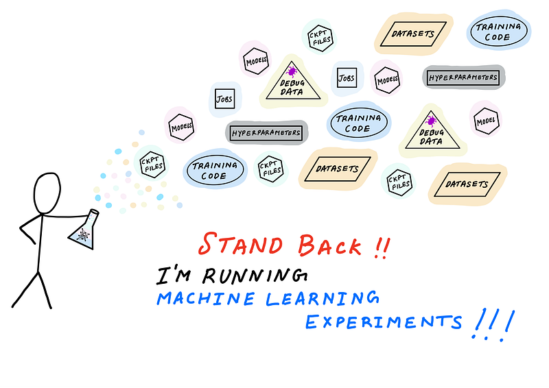
Learn how to organize your machine learning experiments, trials, jobs and metadata with Amazon SageMaker and gain peace of mind

By Shashank Prasanna | Tuesday, July 14, 2020

Illustration by author. Inspired by xkcd.com

The word “experiment” means different things to different people. For scientists (and hopefully for rigorous data scientists), an experiment is an empirical procedure to determine if an outcome agrees or conflicts with some hypothesis. In a machine learning experiment, your hypothesis could be that a specific algorithm (say gradient boosted trees) is better than alternatives (such as random forests, SVM, linear models). By conducting an experiment and running multiple trials by changing variable values, you can collect data and interpret results to accept or reject your hypothesis. Scientists call this process the scientific method.

Regardless of whether you follow the scientific method or not, conducting and managing machine learning experiments is hard. It’s challenging because of the sheer number of variables and artifacts to track and manage. Here’s a non-exhaustive list of things you may want to keep track of:

Parameters: hyperparameters, model architectures, training algorithms
Jobs: pre-processing job, training job, post-processing job — these consume other infrastructure resources such as compute, networking and storage
Artifacts: training scripts, dependencies, datasets, checkpoints, trained models
Metrics: training and evaluation accuracy, loss
Debug data: Weights, biases, gradients, losses, optimizer state
Metadata: experiment, trial and job names, job parameters (CPU, GPU and instance type), artifact locations (e.g. S3 bucket)

As a developer or data scientist, the last thing you want to do is to spend more time managing spreadsheets or databases to track experiments and the associated entities and their relationships with each other.

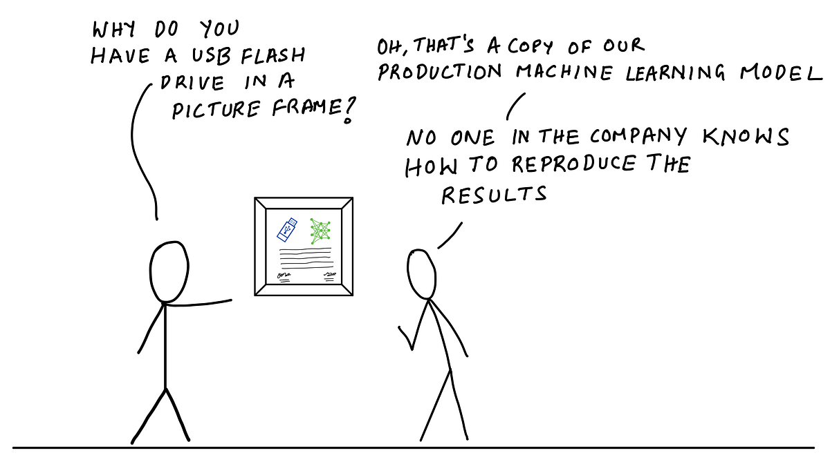
Illustration by author

How often have you struggled to figure out what dataset, training scripts and model hyperparameters were used for a model that you trained a week ago? a month ago? a year ago? You can look through your notes, audit trails, logs and Git commits, and try to piece together the conditions that resulted in that model, but you can never be sure if you didn’t have everything organized in the first place. I’ve had more than one developer tell me something to the effect of “we don’t know how to reproduce our production model, the person who worked on this isn’t around anymore — but it works, and we don’t want to mess with it”.

In this blog post, I’ll discuss how you can define and organize your experiments so that you don’t end up in such a situation. Through a code example, I’ll show how you can run experiments, track experiment data and retrieve it for analysis using Amazon SageMaker Experiments. The data you need about a specific experiment or training job will always be quickly accessible whenever you need it without you having to the bookkeeping.

A complete example in a Jupyter notebook is available on GitHub: https://github.com/shashankprasanna/sagemaker-experiments-examples.git

Anatomy of a machine learning experiment

The key challenge with tracking machine learning experiments is that there are too many entities to track and complex relationships between them. Entities include parameters, artifacts, jobs and relationships could be one-to-one, one-to-many, many-to-one between experiments, trials and entities. Wouldn’t it be nice if you could track everything automatically? That way you can worry less and become more productive, knowing that your experiments are always self-documenting. This is exactly the approach we’ll take.

Let’s start off by introducing a few key concepts. I’ll keep coming back to these throughout the article, so this won’t be the last you’ll hear about them. By presenting these key concepts upfront I hope it will give you a better sense of the relationship between experiments, trials, trial components, jobs, artifacts, metrics and metadata as you go through the example.

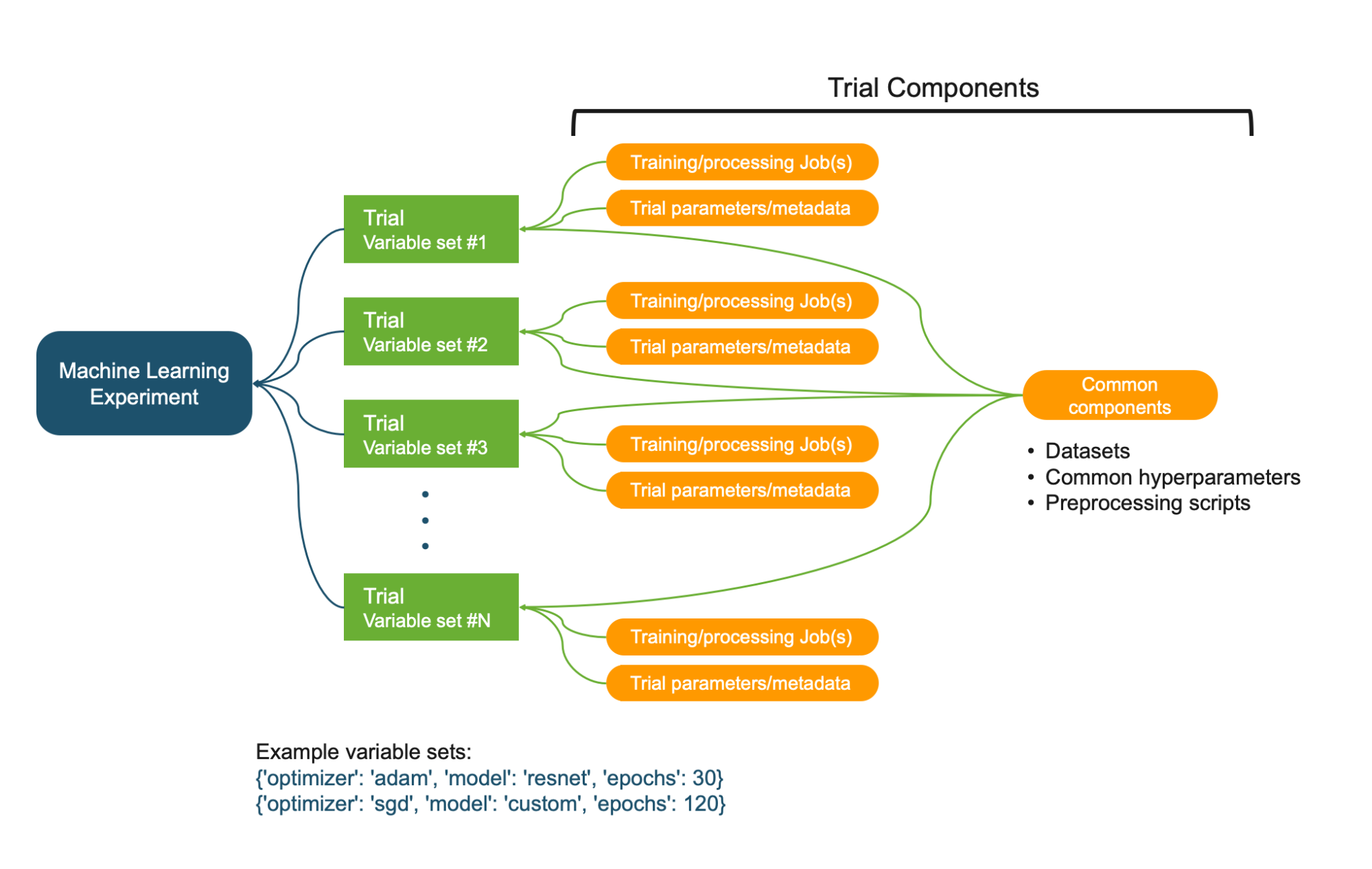
Relationships between Experiment, Trials, and Trial Components. Illustration by author.

Machine learning experiment: A systematic procedure to test a hypothesis (e.g. model A is better than model B, Hyperparameters X has a positive effect on response Y)
Variables: Controllable factors that you vary and measure response (e.g. model architectures, hyperparameters)
Trial: A training iteration on a specific variable set. A variable set could be sampled from an exhaustive set of variable interactions (e.g. model architecture, optimizer, other hyperparameters).
Trial components: Various parameters, jobs, datasets, models, metadata and other artifacts. Trial component can be associated with a Trial (e.g. Training job) or be independent (e.g. metadata)

Properties of an experiment, trial and trial component:

An Experiment is uniquely characterized by its objective or hypothesis
An Experiment usually contains more than one Trial, one Trial for each variable set.
A Trial is uniquely characterized by its variable set, sampled from the variable space defined by you.
A Trial component is any artifact, parameter or job that is associated with a specific Trial.
A Trial component is usually part of a Trial, but it can exist independent of an experiment or trial.
A Trial component cannot be directly associated with an Experiment. It has to be associated with a Trial which is associated with an Experiment.
A Trial component can be associated with multiple Trials. This is useful to track datasets, parameters and metadata that is common across all Trials in an Experiment.

These concepts will become clearer as you go through the example, so don’t worry if you haven’t memorized them. We’ll build out every step starting from creating an experiment.

Managing machine learning experiments, trials, jobs and metadata using Amazon SageMaker

The best way to internalize the concepts discussed so far is through code examples and illustrations. In this example, I’ll define a problem statement, formulate a hypothesis, create an experiment, create trackers for tracking various artifacts and parameters, run Trials and finally analyze results. I’ll do this using Amazon SageMaker Experiments. I’ve made a full working example available for you in the following Jupyter Notebook on GitHub: sagemaker-experiments-examples.ipynb.

The quickest and easiest way to run this notebook is to run it on Amazon SageMaker Studio. SageMaker Studio Notebooks lets you launch a Jupyter notebook environment with a single click, and it includes an experiment tracking pane and visualization capabilities which makes it easier to track your experiments. You can also run this on your own laptop or desktop with Amazon SageMaker python SDK and Amazon SageMaker Experiments packages installed.

Step 1: Formulate a hypothesis and create an experiment

The first step is to define your hypothesis. If you prefer business-speak over academic-speak, you can specify an experiment objective or goal instead. It may be tempting to “just try a bunch of things and pick the best”, but a little effort upfront in defining your problem will give you peace of mind later.

Let’s define an example hypothesis. Your hypothesis takes into account your domain expertise and any preliminary research or observations you’ve made. For example:

Hypothesis: If I use my custom image classification model, it will deliver better accuracy compared to a ResNet50 model on the CIFAR10 dataset

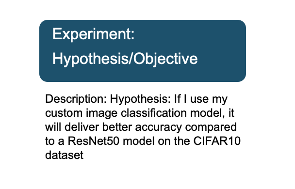
An experiment is uniquely defined by its hypothesis. By stating the hypothesis, you now have a clear path to designing an experiment, selecting the right variables and gathering enough data to accept or reject this hypothesis. Using SageMaker experiments SDK, you can define an experiment as follows. In the description, I include my experiment hypothesis.

The following code creates a SageMaker Experiment:

Step 2: Define experiment variables

An experiment includes a list of variables that you vary across a number of trials. These variables could be hyperparameters such as batch size, learning rate, optimizers, or model architectures or some other factor that you think can have an effect on the response i.e. accuracy or loss in our example. In the field of experimental design, these are also called controlled factors.

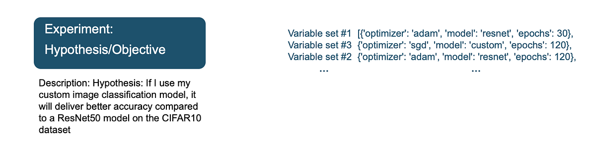
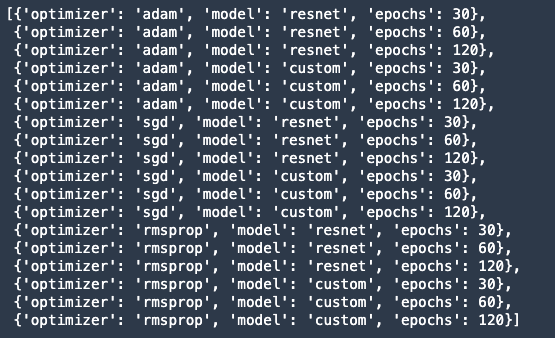
In our example, I want to test the efficacy of our custom neural network architecture, which I believe to be better than off-the-shelf ResNet50. Therefore model architecture is our first variable or controlled factor. I also want to study the effect of other hyperparameters on the response — optimizer (adam, sgd, rmsprop), epochs (high accuracy at fewer epochs). I can define these with the following code.

Output:

Other hyperparameters that are not part of the experiment can be made static (unchanging across trials), so I’ll call them static hyperparameters.

Note: This does not mean that static hyperparameters have no effect on the response. It just means that it’s not a variable you’re controlling in this experiment. There are other factors you can’t control, for example, software bugs, inefficient resource allocation by the operating system, the weather or your mood when running the experiment. These are referred to as uncontrollable factors in the field of experimental design.

Step 3: Tracking experiment datasets, static parameters, metadata

Before I launch several experiment trials and training jobs for each of the hyperparameter options in Step 2, I have to make sure that I also track artifacts and parameters that are common across trials.

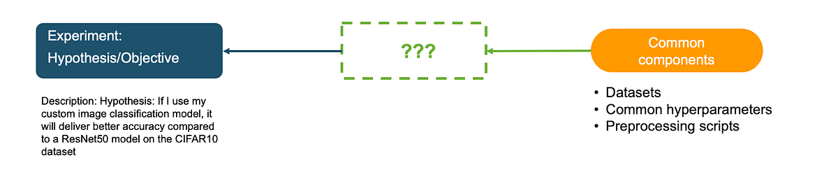
In this example, the following are unchanging across trials:

Static hyperparameters (batch-size, learning-rate, weight-decay, momentum)
List of variables (model architectures and variable hyperparameters)
Training, validation and test dataset
Dataset preprocessing script that generates TFRecord files

You can track anything else you want to be associated with this experiment. The following code creates a tracker called “experiment-metadata” with the above information:

This tracker is a Trial component that is not currently associated with an experiment. Recall that from “Anatomy of a machine learning experiment” a Trial Component cannot be associated with an Experiment directly. It must be associated with a Trial first. In the next section, I’ll associated this common Trial Component with all the Trial in the Experiment.

Step 4: Create Trials and launch training jobs

In Step 2, I created a list of 18 variable sets by varying optimizer, model and epochs. In this step, I’ll loop through these sets and create a Trial and a training job for each set. Here is the approach. For each variable set I will:

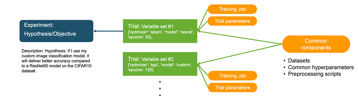
Create a Trial and associate it with the Experiment
Associate the Tracker in Step 3 with this Trial as a Trial Component
Create a new Tracker to track Trial specific hyperparameters and associate it with the Trial as a Trial Component
Create a training job with the Trial specific hyperparameters and associate it with the Trial as a training job Trial Component

The following code excerpt shows how to implement steps a-d above.

The excerpt is shown for illustration only, for a complete example, run this notebook on Github: https://github.com/shashankprasanna/sagemaker-experiments-examples/blob/master/sagemaker-experiment-examples.ipynb

After you run the above code, you’ll see SageMaker spawn multiple training jobs, each associated with its unique Trial.

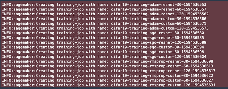
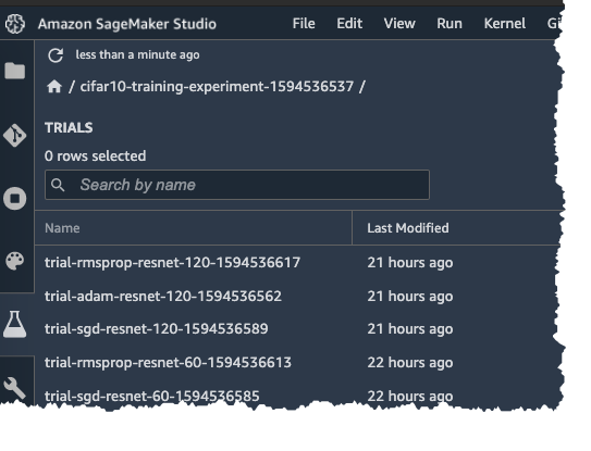
In Amazon SageMaker Studio, you can also view the Experiment Trial on the Experiment pane on the left.

If you double click on one of the Trials and you can see the associated Trial components:

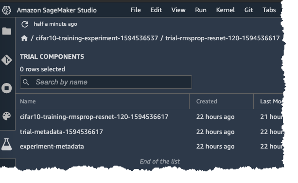
cifar10-training-rmsprop-resnet-120-XXXXX: Trial component for the training job
trial-metadata-XXXXX: Trial Component for the Trial specific hyperparameters
experiment-metadata: Trial Component for entities common to all Trials (Static hyperparameters, list of variables, training, validation and test dataset, dataset preprocessing script)

Step 5: Analyzing Experiment results

After the training jobs have finished running, I can now compare all the Trial runs and draw inferences about the Experiment. With a little bit of effort upfront in carefully defining and organizing your experiments and leveraging services like SageMaker Experiments, you won’t have to spend too much time pulling up reports for analysis by combining multiple digital and analog sources. You can take a vacation or work on a different project while your boss thinks you’re hard at work combing through Git commits, audit trails and entering data into spreadsheets.

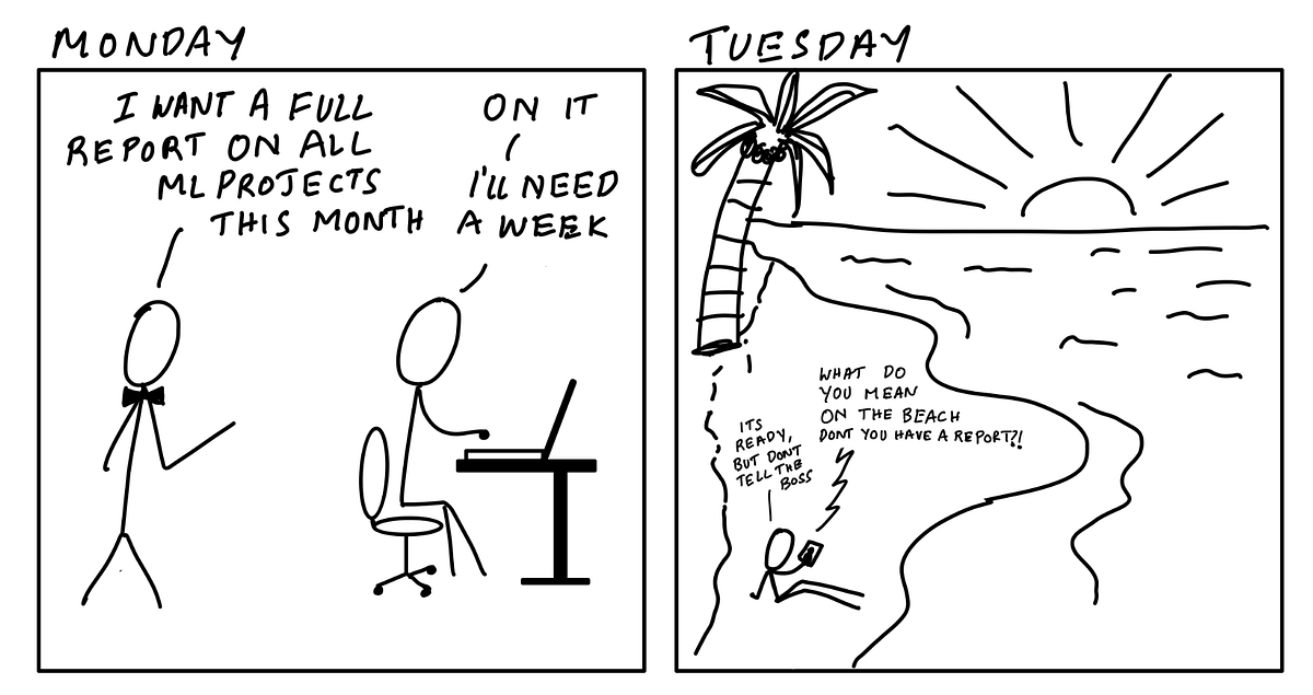
Illustration by author.

In this section, I’ll pull a report on the experiment I just ran. All I need is the name of the experiment, and using the SageMaker Experiments package, I can pull up analytics using the following code:

In the output below, you can see that the (1) best accuracy overall (2) best accuracy @ 60 epochs and (3) best accuracy @ 30 epochs all corresponds to my custom model.

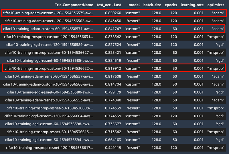
I can use this data to either accept or reject my hypothesis that my custom model delivers better accuracy than ResNet50 for the CIFAR10 dataset. I built this example to illustrate the key concepts of experiment management, and the above data may not be sufficient to draw any conclusions. In which case you can conduct another experiment by updating your hypothesis and variables.

(Bonus) Step 6: Using SageMaker Debugger to visualize performance curves

If you like to dive deep into each training job and analyze metrics, weights or gradient information, you can use SageMaker Debugger. SageMaker Debugger automatically captures some default debug information from every training job, and you can also customize what data should be emitted for later analysis. If you’re interested in debugging machine learning with SageMaker check out my earlier post that does a deep dive on debugging:

Blog post: How to debug machine learning models to catch issues early and often

The smdebug open source library lets you read and analyze debug data. The code below will download validation accuracy for all Trials for each step during training, and plot the 3 top models for 30, 60 and 90 epochs. You can also plot intermediate tensors and gradients during training for further debugging. Check out the above blog post for more details.

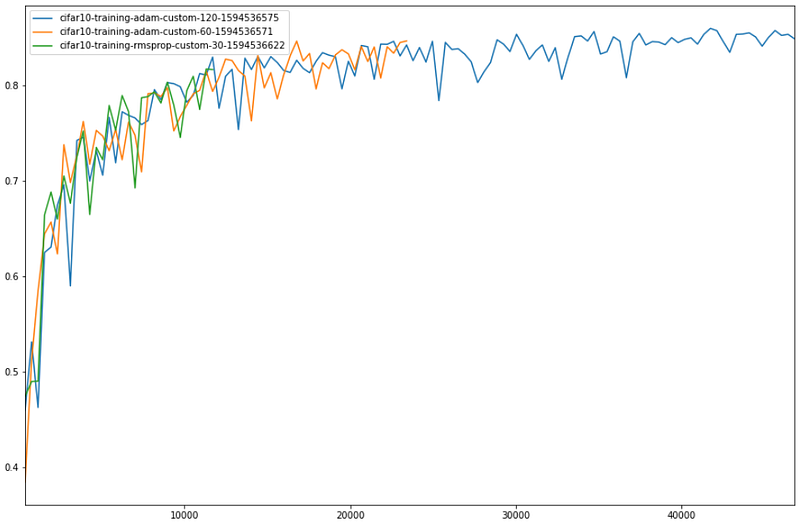
Validation accuracy vs. steps for the top performing model at 30, 60 and 120 epochs

Thanks for reading

We’ve come a long way since the early days of machine learning. From high-quality open-source machine learning frameworks to fully-managed services for training and deploying models at scale, and end-to-end experiment management, there are no shortages of tools no matter what your machine learning needs are. In this blog post, I covered how you can alleviate pains associated with managing machine learning experiments, using Amazon SageMaker. I hope you enjoyed reading. All the code and examples are available on GitHub here:

https://github.com/shashankprasanna/sagemaker-experiments-examples

If you found this article interesting, please check out my other blog posts on machine learning and SageMaker:

If you have questions about this article, suggestions on how to improve it or ideas for new posts, please reach out to me on twitter (@shshnkp), LinkedIn or leave a comment below. Enjoy!